Surfendipity

Attached Code: https://github.com/iainkfraser/PageRank/tree/blogcode

Let's start with a question. How would you order all websites in order of importance? You could order by most popular, most informative or most authoritative.

None of those are truly satisfactory because the question is subjective. It depends on who is asked. For example I would rank technical, comedy and competitive gaming sites highly conversely fashion, gossip and liberal arts sites would rank extremely low. Yet incomprehensible many (majority?) people think the opposite.

So we alter a websites rank depending on the viewer. This is what Google does now but originally googled ranked websites using the PageRank algorithm (named after one of the founders Larry Page). The algorithm takes an objective approach to solving the problem.

Figure 1. Random surfer

We have all been there, you go on the web with a specific purpose and then through a magical Intertubes journey you end up somewhere totally unpredictable. For example I started today searching for the relationship between static code analysis and the halting problem, and I hate to admit ended up on youtube...

Jeez Louise what on earth does that anecdote have to do with PageRank? Its a nice analogy of how PageRank works. Given a user (for example a monkey) that surfs the web by randomly clicking links. The PageRank of a website is the probability of that user landing on the site after a significant number of clicks. This is illustrated in Figure 2.

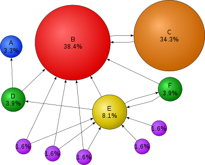
Figure 2. Graph with PageRank values.

So you can think of hyper-links as the source website vouching for the destination website. This explains why website B in Figure 2 is ranked so highly because many sites link to it. In contrast site C is ranked highly even though it has only one incoming link. The reason being its got an incoming link from the big dogg B. Since its likely to land on B it is also likely to land on C.

“Its not what you know or who you know – its who knows you.”

Ok that makes sense and if you're like me you must be wondering how on Gods green earth do you calculate those probabilities? That is what the rest of the article is about. First we need Markov chain models. These model the movement through a stochastic state machines. These are just state machines with transitions based on probabilities like so:

Figure 3. Directed graph to illustrated state transitions

So just to clarify we can move from state A to B with probability of 0.5 and from B to C with 1.0 and so on so forth.

The Markov chain is just a sequence of random variables ( X₁, X₂, … Xn ) that represent a single state. So you can imagine just walking along the graph. So let's say we start at state A. Then the random variable X₁ represents our first step so it is

P( X₁ = A ) = 0.0

P( X₁ = B ) = 0.5

P( X₁= C ) = 0.5

The most important feature of the Markov chain is that the transitions probabilities do not depend on the past. In this article we assume the transitions are constant throughout. So it doesn't matter at all what ridiculous journey you took to get to a state. To predicate the future all you need is the current state and the transitions. So just to reiterate the past is irrelevant on Markov chains.

Right let's represent the state transitions using a transition matrix T . Since the transitions are probabilities we call it a stochastic matrix (technically the total probability of moving from one state to the others is 1 so the rows sum to 1).

So the entry at row i and column j represents the probability of moving from state i to state j. For example T₂₃ is the probability of moving from state B to state C i.e. 1.0.

Why did we bother converting the graph to a matrix. Well it turns out it has a few neat properties. Let's say we started at state A and I asked you what's the probability of moving to state C in two steps?

To answer assume the following notation P(IJ) means the probability of moving from state I to state J in one step (just look up the matrix). So for example P(AB) = 0.5. So the probability of going from A to C in two steps is the probability of going from A to every state (A, B, C) then the probability of going from that state to C. i.e.

Notice that this corresponds to the entry T²_AC. If you try it out for the rest of the entries it turns out that the product of the transition matrix is the probabilities of going from the row to the column in 2 steps. That is T²_ij the probability of going from state i to state j in two steps. If you multiply that by the transition matrix you get the state transitions for 3 steps. So it turns out that Tⁿ is the state transitions for n steps. Really neat huh? I thought so anyway.

Ok let's multiply our transition matrix so we can see the probabilities for two, three, four, five, twenty and one hundred steps:

Something very interesting happens. The entries seem to converge until all the columns values become equivalent. This means that after a certain number of steps it doesn't matter which state you started on. The probability of getting to another state is constant. My mind = blown. So let's try visualise this:

Figure 4. State with converged population distribution.

So let's say we start with a 100 people. Let's use the values of the converged matrix to place people on the graph. So let's put 40% of them on A and another 40% on C. The last 20% can go on B. So move forward one step in the Markov chain.

Half of A will go to B and the other half will go to C. So the new B will have 20% of people. The new C has 20% and the rest of the people from old B which is also 20% therefore the new C has 40%. Finally new state A has all the people from old state C i.e. 40%. Whad'ya know? We are back where we started. So this shows the steady state that the Markov chain converges on. Once we get into this distribution we stay there forever.

So if the small graph used in the example actually represented three websites and the related hyper-links. Then the stabilised values (i.e. the probabilities for each column in converged matrix) represent the PageRank of each website. Sweet!

This blog is already long enough so I'm going to skip over the intuitive proof of convergence. Although Ive put that in the appendix A. I'll just show how we can use the transition matrix to calculate the PageRank.

If we represent the initial distribution (for example of people) using a vector e.g.

That means ¼ of people are in state A and another ¼ in B and the rest ( ½) are in C. If we multiply the transition matrix with the vector. We will get a new vector representing the distribution after the first step. By the same token if we multiply it by an n step transition matrix then the result is the distribution after n steps. So written mathematically, given a transition matrix T, a source distribution s (represented as a row vector) we can calculate the resulting distribution r after n steps using:

r = s . Tⁿ

So we have two very similar concepts but they are not equivalent.

1. After a number of steps the probability of getting to a state is constant regardless of where you start. So no matter what initial distribution you start with you will end up with stable distribution.
2. If you apply a single state transition on the stable distribution you will get the stable distribution.

Let's go through both these points in order. To illustrate point 1 let's pick any random distribution and multiply it with the stable matrix (the converged matrix). So let's say we have 0.3, 0.3 and 0.4 in states A,B and C respectively. Represent it as a row vector and multiply with the converged matrix:

Notice the result distribution is the stable distribution. So intuitively what does this mean? It just means that given the initial distribution and taking it through a significant number of steps we will eventually end up at the stable distribution.

The stable distribution is interesting because once you're in it you remain in that distribution forever . This just a rewording of point 2. So let's illustrate this by multiplying the stable distribution with the initial transition matrix:

Notice we get the stable distribution again. That makes sense because the definition of the stable distribution is one that doesn't change when transitioned. If you try any other distribution on the transition matrix you will not get the same result.

So if you recall from linear algebra an eigenvector is a vector that is only scaled when transformed by a matrix. That is, given a matrix T, a vector s (called eigenvector) and a scalar lambda (called eigenvalue) we have

This looks very similar to our answer above. Except we have a value of lambda as 1 and we are using a row vector (we could change that by transposing both). So it turns out that the stable distribution is the eigenvector of the transition matrix with an eigenvalue of 1.

So moving back to our PageRank algorithm where the transition matrix is a representation of the web and the stable distribution is the PageRank of websites. We can say the PageRank is the eigenvector of the stochastic matrix representing the topology of hyper-links. Wow! that sounds complicated but hopefully we now understand what that means.

Let's generate the algorithm. So our input is the stochastic transition matrix representing the Web. We want the stable distribution (i.e. the eigenvector). Remember a multiplication of any distribution with the convergence matrix will be that stable distribution / eigenvector. So all we have to do is multiply any distribution with our convergent matrix to get the answer.

So the problem reduces to finding the convergent matrix. Well we know to do that we just need to multiply repetitively (take to the exponent) the transition matrix until it converges. So let x be our initial distribution. Just set it to 1/n where n is the number of components in the vector (i.e. websites). And we have the following formula to calculate the eigenvector: 

Huh? bear with me. Let's expand this out:

So by doing it in this order we can skip a few operations. We can do vector-matrix product instead of matrix-matrix product which has far fewer operations. So the last and final question is when do we stop? when we hit the stable distribution (eigenvector). That is when: 

So let's convert this into a floating point friendly algorithm:

 /* Inputs are  
 * n = number of websites   
 * T = is a n x n transition matrix  
 */  
 vector x = { 1/n, 1/n, ..., 1/n }    // initial distribution  
 do {  
    old = x   
    x = x * T  
    delta = | x - old |  
 } while( delta > EPISILON );  

So once the algorithm is complete, x will be the stable distribution, eigenvector and the PageRank of the web.

So its been a pretty lengthy article for such little code. Always the way with Maths heavy algorithms. For more information on PageRank read "The PageRank Citation Ranking: Bringing Order to the Web" and on Markov chains I highly recommend "Finite Markov Chains and Algorithmic Applications" by Olle Häggström.

So Appendix A has a high-level explanation for convergence. Then Appendix A shows how Google converts the web graph into a Google matrix so that it has a convergent property.

Right I applied the algorithm to the request for comments (RFC) and used citations as links/edges. The PageRank of all RFCs (at the time of writing) in descending order:

https://github.com/iainkfraser/PageRank/blob/master/rfc_pagerank_with_titles.txt

That's all folks - PEACE!

Appendix A - Convergence

I'm going to very briefly describe state transition restrictions that allow convergence. Then i'll explain intuitively why convergence occurs. If you want to learn more about Markov Chains in more detail then refer to a book, it's a subject in its own right.

Theroem: Any irreducible and aperiodic Markov chain has exactly one stationary distribution. 

Before I explain irreducible and aperiodic let me say the converse isn't true. Not being irreducible and aperiodic does not mean there isn't a stationary distribution it just means there may not be. So irreducible and aperiodic chains are interesting because we are guaranteed to have stationary distribution (and therefore a PageRank).

An irreducible graph means there is always a way to get from one state to another eventually. If you can't you call it reducible. Figure 5. has some example illustrations.

Figure 5. The two chains on the left are reducible and the one on the right is irreducible

By the way its called reducible because you can split into two or more separate graphs and model those using Markov chains. So its quite obvious there can't be a stationary distribution because remember the stationary distribution means: the probability of getting from any state to a certain state is constant. So clearly if you can't get to a state the probabilities can't be the same because some states can reach but other(s) cannot.

Figure 6. The two on the right are aperiodic and the left has a period of of 2.

Aperiodic is a bit more difficult to explain. So I'm going to explain it with an example, again read one of the Markov chains books for the formal definition (quickly its the greatest common divisor of the number of steps to get back to the same state).

So look at example  in Figure 6a. If you place all one hundred people on S1. Then if we do the next step they all move to S2  (so none on S1). Then they all move back to S1 and so on and so forth. So clearly its never going to converge because it oscillates. It has a period of 2, because getting back to state S1 takes a minimum of 2 steps.

Compare that with Figure 6c which is aperiodic. So S1 is trivial because we can get straight back to S1 in one step. But S2 we can get back in 2,3,4,5,7... steps. Why isn't that periodic? Let's run through an instance of a Markov chain. So all 100 people move from S2 to S1. Then 50 go back S2 and the other 50 stay on S1. Now look at this distribution (which originally started with 100 on s2) we can get back to S2 now in 1 step forever. Ergo its not periodic.

So let's get onto a intuitive description of the proof. If the graph is aperiodic and irreducible then eventually (after a number of steps) every value in the transition matrix will be between 0 and 1 exclusively (i.e. not 0 or 1). Because there is a way to get from any state to any other state.

Figure 7. Probability of moving to B in one step

So let's start thinking of a hypothetical graph shown in Figure 7. I was going to use variables for transition probability but I think numbers are simpler to understand. So if we were playing a game and wanted to get to B in one step we would start at C and if we didn't want to get to B we would start at A.  How about two steps? 

Figure 8. Probability of moving to B in two steps

So if I asked you to try get to B, what would you say? B->C->B right. Because we already know ending with C -> B is the optimum for one step. So we want the optimum something to C which is B. So the optimum odds of landing on B for 2 steps is 0.54. Notice that the odds are worse than just the single step.

Now if I asked you try to avoid getting to B in two steps what would you say? Well again we want to pick the most likely of landing on A->B (the least likely single step) so we would choose A->A->B which has overall odds of 0.18. Notice again these odds are greater (so in response to the question worst) than the single step.

Figure 9. Probability of A->B in three steps. Notice the minimum is increasing

This illustrates why convergence works. The maximum and minimum probabilities of getting to B will be in the first step. Because in the next step the probability of getting to the maximum step is not 1 so its going to lose a bit (to the other branches). And the probability of getting to the minimum step is also not 1 so we will gain a bit (by the other branches). 

Through induction (due to recursive nature of the steps) we can show that after each step the minimum will raise and the maximum will fall until they eventually converge. Therefore no matter where you start you have the same probability of getting to the destination (B in this case).

It should now make sense why you don't want 1 or 0 entries in the matrix forever. Because that means the maximum or minimum doesn't have to fall or raise and thus converge. 

Appendix B – Google Matrix

So we need the Markov chain to be irreducible and aperiodic to guarantee that there is a stable distribution (see Appendix 1). An easy way to do that is to have a link from every state to every other state.

So how can we transform the hyper-link graph into this type of graph. Because clearly every website doesn't link every other website. The way Google does it, is to imagine that the random surfer may get bored and when that happens they randomly teleport to random website.

So how do we apply this logic to the transition matrix? Well we need a probability of the user getting bored call d (for damping) which is usually set to 0.85 (the clever dudes at Google figured this number out). Then we can convert the transition matrix to:

So the dT just dampens all the links due to the chance of getting more bored. Then there is a chance of ( 1 – d ) divided by the number of sites of randomly teleporting to another site. So we need to add that to every entry in the matrix which is what ee^T (generates a n x n matrix of all ones using outer product).